Source: Time Series in Python — Part 2: Dealing with seasonal data | by Benjamin Etienne | Towards Data Science

Benjamin Etienne

In the first part, you learned about trends and seasonality, smoothing models and ARIMA processes. In this part, you’ll learn how to deal with seasonal models and how to implement Seasonal Holt-Winters and Seasonal ARIMA (SARIMA).

Getting the data

We’ll use the “Monthly milk production” data:

import requests
import pandas as pd
import json
import matplotlib.pyplot as plt
import matplotlib.dates as mdates
%matplotlib inline
plt.style.use('Solarize_Light2')

r = requests.get('https://datamarket.com/api/v1/list.json?ds=22ox')
jobj = json.loads(r.text[18:-1])
data = jobj[0]['data']
df = pd.DataFrame(data, columns=['time','data']).set_index('time')
train = df.iloc[:-24, :]
test = df.iloc[-24:, :]
train.index = pd.to_datetime(train.index)
test.index = pd.to_datetime(test.index)
pred = test.copy()
df.plot(figsize=(12,3));
plt.title(jobj[0]['title']);

Seasonal decomposition (TLS)

In the previous part, I talked briefly about seasonal decomposition. The idea beneath seasonal decomposition is to state that any series can be decomposed in a sum (or a product) of 3 components: a trend, a seasonal component, and residuals.

In our case, we’ll use the seasonal_decompose function provided by statsmodels:

The trend component is an increasing curve which seems to reach a plateau and eventually decrease at the end. This is a useful information when we will remove the trend to stationarize the data.

Stationarizing the data

Dealing with the trend

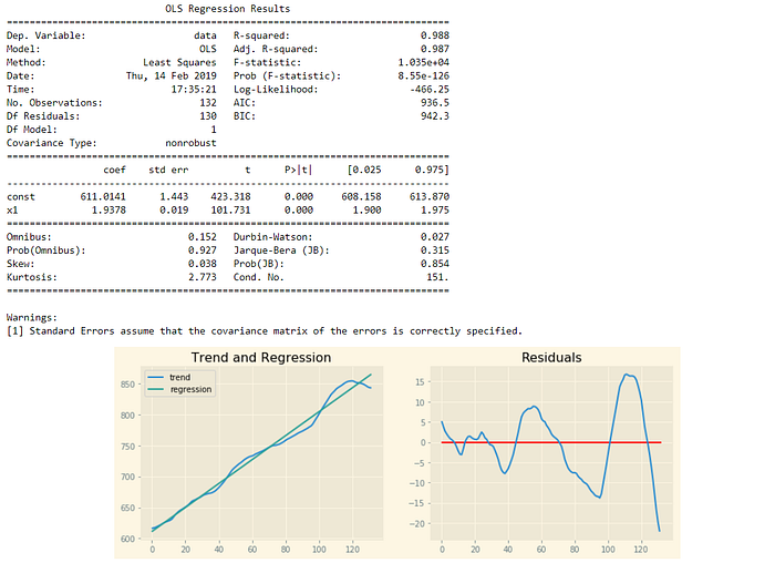
Based on our decomposition, we see that the trend is following an upwards movement before plateauing (and maybe decreasing) at the end. In order to remove the trend, we will try an original approach, consisting in regressing the trend given by the STL decomposition. We will then try, if the regression if satisfying, to “deflate” the series by substracting the obtained regression from the original series.

import statsmodels.api as sm
from statsmodels.api import OLS

x, y = np.arange(len(decomposition.trend.dropna())), decomposition.trend.dropna()
x = sm.add_constant(x)
model = OLS(y, x)
res = model.fit()
print(res.summary())
fig, ax = plt.subplots(1, 2, figsize=(12,6));
ax[0].plot(decomposition.trend.dropna().values, label='trend')
ax[0].plot([res.params.x1*i + res.params.const for i in np.arange(len(decomposition.trend.dropna()))])
ax[1].plot(res.resid.values);
ax[1].plot(np.abs(res.resid.values));
ax[1].hlines(0, 0, len(res.resid), color='r');
ax[0].set_title("Trend and Regression");
ax[1].set_title("Residuals");

The r-squared coefficient from our regression is quite good (0.988), but looking at the residuals we notice that their variance increase from left to right. This is a sign of heteroskedasticity. You can look up the exact definition by yourself, just keep in mind that this is not good and that something is missing in our model. We’ll abandon the idea of regressing the trend as it requires too much effort for now.

Dealing with the trend, ep.2

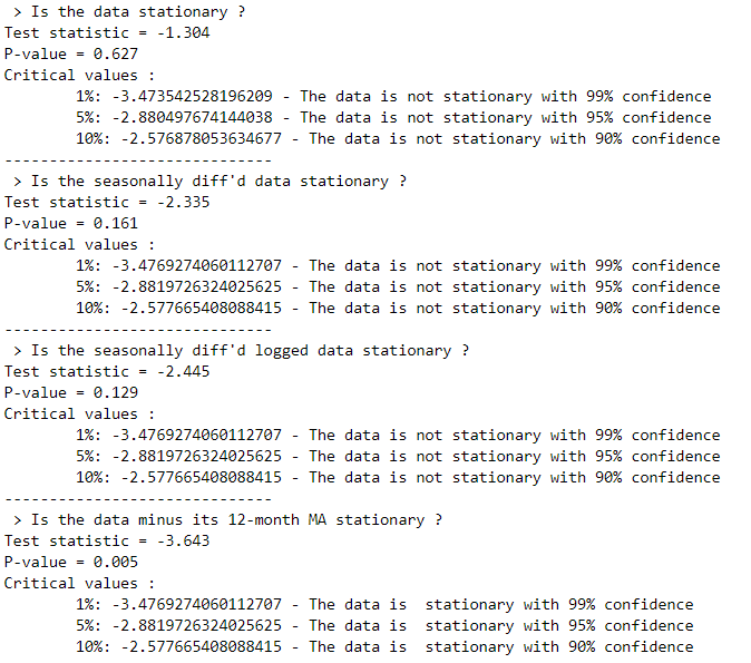
Our series still needs stationarizing, we’ll go back to basic methods to see if we can remove this trend. We’ll operate in several steps :

• ADF test on raw data to check stationarity
• ADF test on the 12-month difference
• ADF test on the 12-month difference of the logged data
• ADF test on the data minus its 12-month moving average

If you need the code, refer to the first part to learn how to conduct an ADF test

Let’s confirm that the data minus its 12-month MA is stationary with a KPSS test :

The test statistic is below the thresholds, therefore our series is stationary (recall that for the KPSS test, the null hypothesis is that the series is stationary).

Fitting a Holt-Winter’s Seasonal Smoothing model

Remember from the first part that a Holt-Winter’s model has several parts : a level, a trend, and in the case of a seasonal smoothing, a seasonal component. The math behind this is a bit hard so I won’t put it here, just remember the three components above. Here is what we get after fitting our model :

The model without damping seems to perform better, as the AIC is lower.

Seasonal ARIMA

Good old ARIMA is back, but this time we’ll add a seasonal component to it ! A SARIMA model is composed of two parts: a non-seasonal part and a seasonal part. If you remember the previous part, the non-seasonal part is composed of an AR(p) term, a MA(q) term, and a I(d) term, and we write ARIMA (p, d, q). Well it’s the same for the seasonal part !
Our SARIMA is noted ARIMA (p, d, q)x(P, D, Q).

Question : how do we determine all these p, d, q, P, D, Q ?

Each time you hear “ARIMA”, think “ACF/PACF”.

With the ACF and PACF plots, we’ll be able to guess reasonable values for our parameters. Let’s plot the ACF and PACF plots of our stationarized data :

The data is clearly not stationary given the slow decay of spikes observed in the ACF. This is a sign that we should take an additional difference for x:

Our series is now stationary. To sum up, we have :

• taken a 12-lag difference of the stationarized series. This corresponds to a “1-seasonal-lag” difference.
• taken a 1-lag difference of the 12-lag differenced series. This corresponds to a non-seasonal difference order of 1.

This gives us an SARIMA(?, 1, ?)x(?, 1, ?).

What about the AR and MA terms ?

Well, we know that there are still significant spikes in the ACF and PACF, so we could decide to add AR terms as well as MA terms. Which one should we start with ? For this time, we’ll use a grid search over the possible combinations on AR and MA terms (limited to a maximum order of 2)…

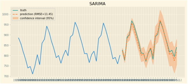
When running different configurations, the lowest AIC is obtained with a SARIMA(0, 1, 2)x(0, 1, 2).

With the plot_diagnotics() command, we can show the residuals and check their normality ( — remember, the residuals should be normally distributed (zero mean and unitary variance) and be uncorrelated).

Notice how the normal Q-Q plot and the histogram show that our residuals follow a normal distribution (we could use additional tests to test for normality, such as Ljung-Box). The correlogram also shows that the residuals are uncorrelated !